Signal Subgraph Estimators

This tutorial will introduce the following signal-subgraph estimators:

• Incoherent subgraph estimator

• Coherent subgraph estimator

import graspologic.subgraph as sg
import matplotlib.pyplot as plt
import numpy as np

/home/runner/.cache/pypoetry/virtualenvs/graspologic-pkHfzCJ8-py3.10/lib/python3.10/site-packages/tqdm/auto.py:21: TqdmWarning: IProgress not found. Please update jupyter and ipywidgets. See https://ipywidgets.readthedocs.io/en/stable/user_install.html
  from .autonotebook import tqdm as notebook_tqdm

Preliminaries

The general graph model is characterized by \(M_V(m,s;\pi,p,q)\), where:

\(V\) - the number of vertices in the graph

\(n\) - the number of graph samples

\(s\) - the number of edges that must be present in the subgraph

\(m\) - the number of vertices that each edge in the subgraph must be incident to

\(\pi\) - the probability of a graph sample being of class 1

\(p\) - the probability of edges in the signal-subgraph, conditioned on Class 0

\(q\) - the probability of edges in the signal-subgraph, conditioned on Class 1

The signal-subgraph is a subset of edges with distinct class-conditional likelihood parameters. The signal-subgraph estimator evaluates a test statistic for each edge in the graph and selects \(s\) edges with the lowest test statistic, where \(s\) is the desired size of the signal-subgraph.

The estimator that is used to find the signal-subgraph determines certain properties of the resulting subgraph. Both estimators use \(s\) to determine the size of the resulting subgraph. \(m\) is only used for the coherent estimator, which constrains the subgraph to \(m\) vertices.

Incoherent Signal-Subgraph Estimator

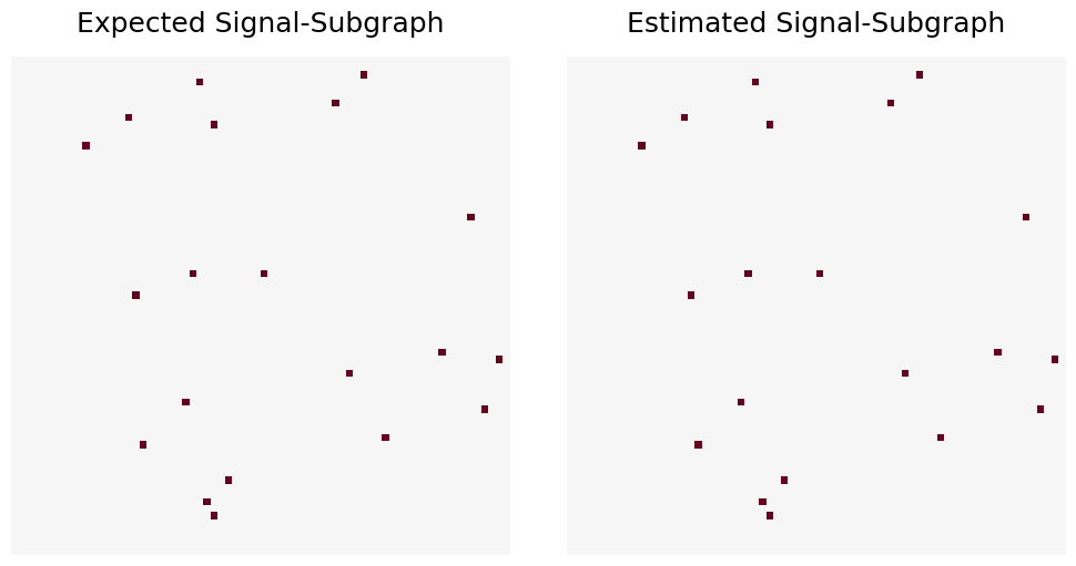
For this example we will randomly select 20 edges from a graph with 70 vertices. These edges will have distinct class-conditional edge probabilities, and the graphs will be sampled from the model \(M_{70}(20; 0.5, 0.8, 0.1)\), with \(n = 100\).

from graspologic.plot import heatmap

verts = 70
sedges = 20
pi = 0.5
p = 0.8
q = 0.1
nsamples = 100

np.random.seed(8888)
classlabels = np.zeros(nsamples, dtype=int)
classlabels[1::2] = 1

sigsubindex = np.random.choice(verts ** 2, sedges, replace=False)
vect = p * np.ones(verts ** 2)
vect[sigsubindex] = q
vect = np.reshape(vect, (verts, verts))
expected = np.where(vect == q, 1, 0)

blank = vect[:, :, None] + np.zeros(int(nsamples / 2))
A = p * np.ones((verts, verts, nsamples))
A[:, :, 1::2] = blank
A = np.random.binomial(1, A)

sigsub = sg.SignalSubgraph()
sigsub.fit_transform(graphs=A, labels=classlabels, constraints=sedges)

estimatesigsub = np.zeros((verts, verts))
estimatesigsub[sigsub.sigsub_] = 1

fig, ax = plt.subplots(ncols=2, figsize=(10, 5), constrained_layout=True)
heatmap(expected, ax=ax[0], cbar=False, title="Expected Signal-Subgraph")
_ = heatmap(estimatesigsub, ax=ax[1], cbar=False, title="Estimated Signal-Subgraph")

Note that because \(p\) and \(q\) are sufficiently distinct and \(n\) is sufficiently large, the Expected and Estimated signal-subgraphs should match exactly.

Incoherent Signal-Subgraph Estimator

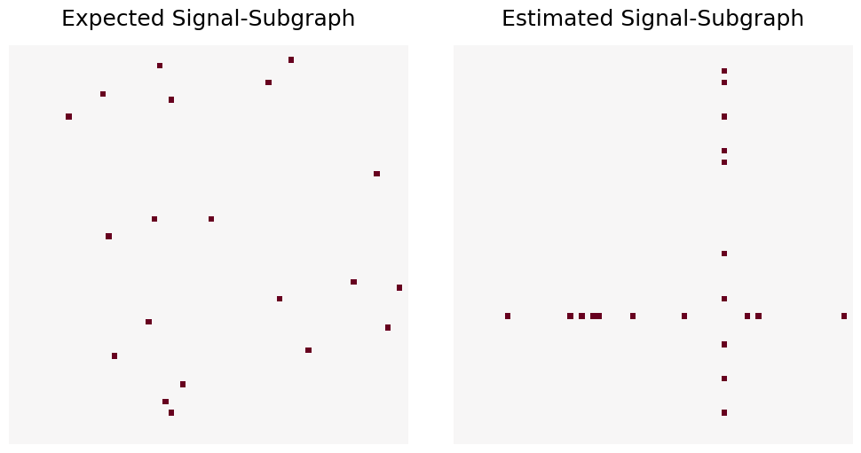
Once again, we will randomly select 20 edges from a graph with 70 vertices. These edges will have distinct class-conditional edge probabilities, but the graphs will be sampled from the model \(M_{70}(1, 20; 0.5, 0.8, 0.1)\), with \(n = 100\).

The estimated signal-subgraph will have 20 edges, constrained so that each edge must be incident to the same vertex. First, we will use the same expected signal-subgraph as the previous example.

np.random.seed(8888)
classlabels = np.zeros(nsamples, dtype=int)
classlabels[1::2] = 1

sigsubindex = np.random.choice(verts ** 2, sedges, replace=False)
vect = p * np.ones(verts ** 2)
vect[sigsubindex] = q
vect = np.reshape(vect, (verts, verts))
expected = np.where(vect == q, 1, 0)

blank = vect[:, :, None] + np.zeros(int(nsamples / 2))
A = p * np.ones((verts, verts, nsamples))
A[:, :, 1::2] = blank
A = np.random.binomial(1, A)

sigsub = sg.SignalSubgraph()
sigsub.fit_transform(A, classlabels, [20, 1])

estimatesigsub = np.zeros((verts, verts))
estimatesigsub[sigsub.sigsub_] = 1

fig, ax = plt.subplots(ncols=2, figsize=(10, 5), constrained_layout=True)
heatmap(expected, ax=ax[0], cbar=False, title="Expected Signal-Subgraph")
_ = heatmap(estimatesigsub, ax=ax[1], cbar=False, title="Estimated Signal-Subgraph")

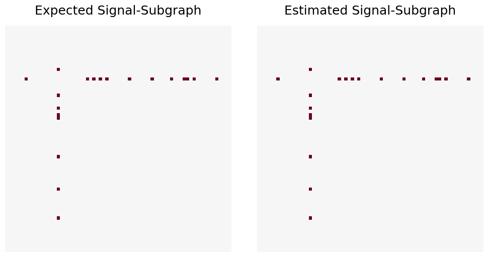
Notice how the coherent estimator constrains the estimated signal-subgraph to 20 edges that are incident to 1 vertex with the best total significance values. Now, we will try an expected signal-subgraph that is also limited to one vertex.

mverts = 1

np.random.seed(7777)
classlabels = np.zeros(nsamples, dtype=int)
classlabels[1::2] = 1

m = np.random.choice(verts, mverts)
vect = p * np.ones(2 * verts * mverts - (mverts ** 2))
vect[np.random.choice(len(vect), sedges, replace=False)] = q

blank = p * np.ones((verts, verts))
blank[m, :] = np.nan
blank[:, m] = np.nan
blank[np.isnan(blank)] = vect
expected = np.where(blank == q, 1, 0)

blank = blank[:, :, None] + np.zeros(int(nsamples / 2))
A = p * np.ones((verts, verts, nsamples))
A[:, :, 1::2] = blank
A = np.random.binomial(1, A)

sigsub = sg.SignalSubgraph()
sigsub.fit_transform(graphs=A, labels=classlabels, constraints=sedges)

estimatesigsub = np.zeros((verts, verts))
estimatesigsub[sigsub.sigsub_] = 1

fig, ax = plt.subplots(ncols=2, figsize=(10, 5), constrained_layout=True)
heatmap(expected, ax=ax[0], cbar=False, title="Expected Signal-Subgraph")
_ = heatmap(estimatesigsub, ax=ax[1], cbar=False, title="Estimated Signal-Subgraph")

Now that the expected signal-subgraph is constrained to the coherent signal-subgraph model, the Expected and Estimated signal-subgraphs are exactly equal.