Correlated Graph Pairs

import graspologic
import matplotlib.pyplot as plt
import numpy as np
%matplotlib inline

/home/runner/.cache/pypoetry/virtualenvs/graspologic-pkHfzCJ8-py3.10/lib/python3.10/site-packages/tqdm/auto.py:21: TqdmWarning: IProgress not found. Please update jupyter and ipywidgets. See https://ipywidgets.readthedocs.io/en/stable/user_install.html
  from .autonotebook import tqdm as notebook_tqdm

The correlated Graph Pairs Model means that we generate a graph pair with some correlation. We define the probability of observing the same edge in both graphs by adjusting the correlation values and sampling the graph pairs.

ER correlation graph pair

There are different ways to define the probability matrix of the first graph. The ER model is a simple example. We assume that each edge for all pairs of vertices is sampled independently from each other edge.

ER_CORR(n, p, r) - this model specifies the number of vertices, \(n\), the probability of an edge existing between a given pair of vertices, \(p\), and the correlation value between the two, \(r\).

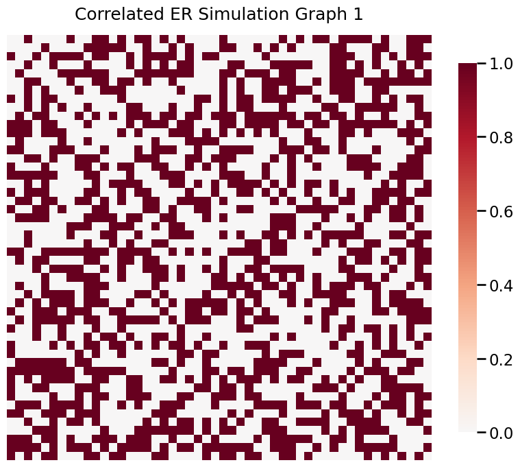
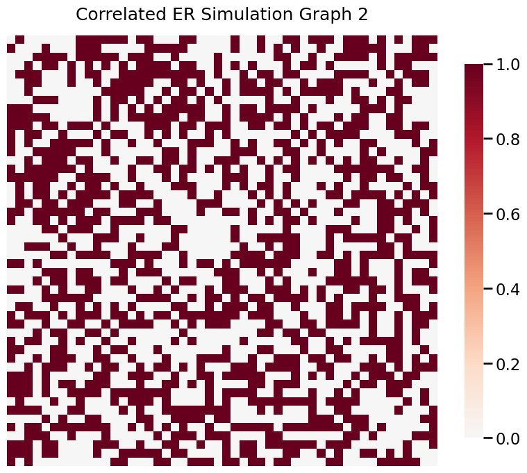
Below, we sample a graph pair with the ER model (undirected and no self-loops) \(G_1, G_2 \sim ER\_{CORR}\,(50, 0.5, 0.3)\).

from graspologic.simulations import er_corr

n = 50
r = 0.3
p = 0.5

np.random.seed(2)
G1, G2 = er_corr(n, p, r, directed = False, loops = False)

Visualize the graphs using heatmap

from graspologic.plot import heatmap
heatmap(G1, title = 'Correlated ER Simulation Graph 1')
_ = heatmap(G2, title = 'Correlated ER Simulation Graph 2')

SBM correlated graph pair

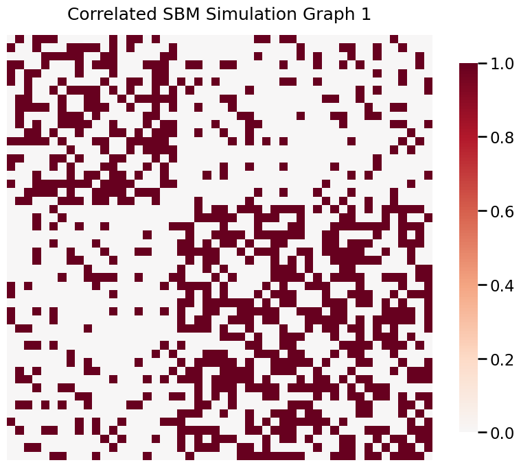
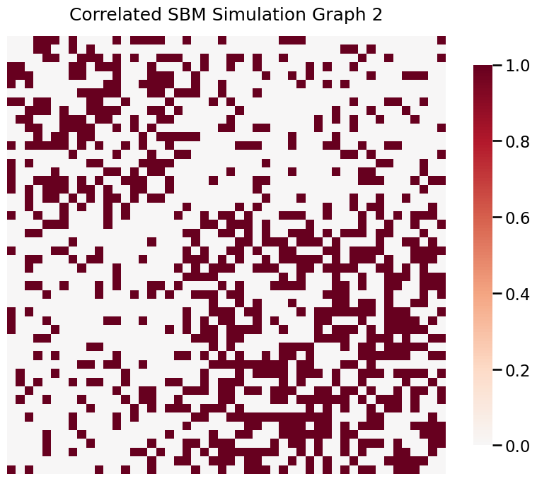
Stochastic block models tend to produce graphs containing communities: subsets characterized by being connected with one another with particular edge densities. We can define the partitioned matrix with different probabilities of having edges and the correlation values between the two.

Below, we sample a two-block SBM graph pair (undirected and no self-loops) G1 and G2 with the following parameters:

\begin{align*} n &= [20, 30]\\ p &= \begin{bmatrix} 0.5 & 0.2\\ 0.2 & 0.5 \end{bmatrix}\\ r &= 0.3 \end{align*}

from graspologic.simulations import sbm_corr

np.random.seed(3)
n = [20, 30]
p = [[0.5, 0.2], [0.2, 0.5]]
r = 0.3

G1, G2 = sbm_corr(n, p, r, directed=False, loops=False)

Visualize the graphs using heatmap

heatmap(G1, title = 'Correlated SBM Simulation Graph 1')
_ = heatmap(G2, title = 'Correlated SBM Simulation Graph 2')