Aligning

align is a module that can be used to align two different datasets. In particular, all three currently existing classes, namely SignFlips, regular OrthogonalProcrustes, and SeedlessProcrustes are aimed at correcting an orthogonal transformation of the data, the exact form of which is unknown. The motivation for this are orthogonal non-identifiabilities, which are common when dealing with various embedding methods, whether in statistical graphs or other domains. Noted that if two graphs are embedded using omnibus embedding - they don’t need to be aligned.

Recall that an orthogonal matrix is any matrix \(Q\) such that \(Q^T Q = Q Q^T = I\). For all alignment methods, the main idea is to infer an orthogonal matrix \(Q\) from the input data sets \(X\) and \(Y\), and subsequently use \(Q\) in order to align \(X\) to \(Y\), by transforming \(X\) as \(\hat{X} = X Q\). The major differences among classes in align come from the settings in which they are applicable, as well as additional assumptions made on the matrix \(Q\).

import numpy as np
import matplotlib.pyplot as plt
from graspologic.plot import heatmap
from scipy.stats import special_ortho_group, ortho_group

%matplotlib inline

Simple rotation example

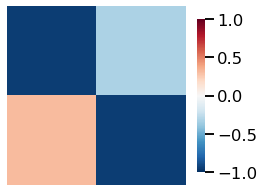
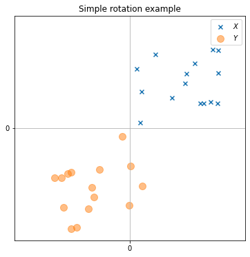
First, let’s build two simple datasets \(X\) and \(Y\), with all entries of \(X\) coming from the \(Uniform(0, 1)\) distribution, and \(Y\) is a copy of \(X\), and subsequently rotated around the origin, using the randomly generated matrix \(Q\), displayed below:

np.random.seed(314)
X = np.random.uniform(0, 1, (15, 2))
Q = special_ortho_group.rvs(2)
Y = X @ Q

heatmap(Q, figsize=(4,4), vmin=-1, vmax=1)
Q

array([[-0.94924938, -0.31452442],
       [ 0.31452442, -0.94924938]])

fig, ax = plt.subplots(1, 1, figsize=(6, 6))
ax.set_title("Simple rotation example")
ax.scatter(X[:,0], X[:,1], label=r"$X$", marker='x')
ax.scatter(Y[:,0], Y[:,1], label=r"$Y$", s=100, alpha=0.5)
ax.set(xlim=(-1.20, 1.20), ylim=(-1.20, 1.20))
ax.set_xticks([0])
ax.set_yticks([0])
ax.legend()
ax.grid();

SignFlips

SignFlips assumes that \(Q\) is not only orthogonal, but also diagonal, which constraints to matrices with \(\pm 1\) along the diagonal and \(0\) everywhere else. In essence, it flips the dataset along some axes such that the two datasets end up in the same orthant (generalized quadrant). Which quadrant the dataset is “located” in is defined by some criterion, which is the dimension-wise medians by default. If the dataset needs to flip along some dimension, the corresponding entry in \(Q\) will be \(-1\), and \(1\) otherwise.

from graspologic.align import SignFlips
aligner_SF = SignFlips()
X_prime_SF = aligner_SF.fit_transform(X, Y)

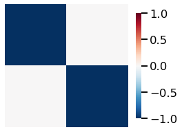
Since \(X\) is entirely in the first quadrant, its dimension-wise medians in both dimensions are greater than \(0\). Meanwhile \(Y\) is predominantly in the third quadrant, so its dimension-wise medians are all smaller than \(0\). Thus \(X\) needs to be flipped both along the x-axis and y-axis in order for two datasets to arive to the same quandrant. So, the \(Q_{SF}\) that the algorithm finds is

heatmap(aligner_SF.Q_, figsize= (4,4), vmin=-1, vmax=1)
aligner_SF.Q_

array([[-1,  0],
       [ 0, -1]])

fig, ax = plt.subplots(1, 1, figsize=(6, 6))
ax.set_title("Simple rotation example, Sign Flips")
ax.scatter(X[:,0], X[:,1],
           label=r"$X$", marker='x')
ax.scatter(Y[:,0], Y[:,1],
           label=r"$Y$", s=100, alpha=0.5)
ax.scatter(X_prime_SF[:,0],
           X_prime_SF[:,1],
           label=r"$X_{SF}$",
           marker='$F$')
ax.set(xlim=(-1.20, 1.20), ylim=(-1.20, 1.20))
ax.set_xticks([0])
ax.set_yticks([0])
ax.legend()
ax.grid();

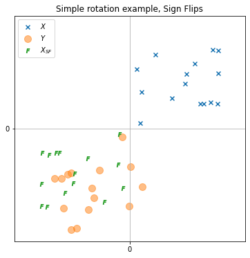
SignFlips correctly brings \(X\) to the third quadrant, yet the alignment is imperfect, as it is a heuristic-based method. Note that it does not assume that there is any sort of matching between the entries of \(X\) and \(Y\). Indeed, the two datasets need not even be of the same size.

This class can also be used to bring the dataset to the first orthant, if one provides the identity matrix as the second dataset.

OrthogonalProcrustes

OrthogonalProcrustes obtains \(Q_{OP}\) by solving the classic orthogonal procrustes problem.

Orthogonal Procrustes problem is a matrix approximation problem in linear algebra, as one is asked to find a orthogonal matrix \(Q\), which could most closely map the given matrix \(X\) to another given matrix \(Y\). Formally it seeks to find a matrix \(Q_{OP}\) such that \(|| X Q_{OP} - Y ||_F\) is minimized.

Since, this formulation strongly relies on the correspondence between the rows of the given matrices, this class can only be applied when the entery datasets \(X\) and \(Y\) have the equal shape (\(n\), \(d\)), and the \(i^{th}\) entry in \(X\) is assumed to be the same value as vertex \(i^{th}\) entry of \(Y\), up to some noise. In graph setting, this means that the latent positions of the two graphs are equivalent.

OrthogonalProcrustes has a widely known closed form solution. Indeed, this class simply wraps scipy.linal.orthogonal_procrustes().

from graspologic.align import OrthogonalProcrustes
aligner_OP = OrthogonalProcrustes()
X_prime_OP = aligner_OP.fit_transform(X, Y)

Note that that \(Q_{OP}\) is a generic orthogonal matrix, not a diagonal one.

heatmap(aligner_OP.Q_, figsize= (4, 4), vmin=-1, vmax=1)
aligner_OP.Q_

array([[-0.94924938, -0.31452442],
       [ 0.31452442, -0.94924938]])

fig, ax = plt.subplots(1, 1, figsize=(6, 6))
ax.set_title("Simple rotation example, OrthogonalProcrustes")
ax.scatter(X[:,0], X[:,1], label=r"$X$", marker='x')
ax.scatter(Y[:,0], Y[:,1], label=r"$Y$", s=100, alpha=0.5)
ax.scatter(X_prime_OP[:,0],
           X_prime_OP[:,1],
           label=r"$X_{OP}$",
           marker='$O$')
ax.set(xlim=(-1.20, 1.20), ylim=(-1.20, 1.20))
ax.set_xticks([0])
ax.set_yticks([0])
ax.legend()
ax.grid();

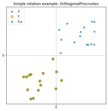
As expected, OrthogonalProcrustes obtains an exact solution when \(X\) is a rotated copy of \(Y\).

SeedlessProcrustes

SeedlessProcrustes is an algorithm that extends regular Procrustes to a case when there is no known correspondence between the entries. In fact, it can be used even when the number of entries between the two datasest is different.

Formally, if \(X\) has \(n\) entries, and \(Y\) has \(m\) entries, it tries to solve for an orthogonal matrix \(Q_{SP}\), and an \(n \times m\) matrix \(P\), with a special condition that rows sum to \(1/m\), and columns sum to \(1/n\), such that the quantity \(|| X Q_{SP} - P Y ||_F\) is minimized.

Unlike the regular procrustes, this does not have a known closed form solution. SeedlessProcrustes tries to solve this optimization problem via an iterative algorithm that alternates optimal transport and regular procrustes. See the Notes section of the SeedlessProcrustes references for more details on this algorithm.

from graspologic.align import SeedlessProcrustes
aligner_SP = SeedlessProcrustes()
X_prime_SP = aligner_SP.fit_transform(X, Y)

heatmap(aligner_SP.Q_, figsize=(4,4), vmin=-1, vmax=1)
aligner_SP.Q_

array([[-0.94472887, -0.32785266],
       [ 0.32785266, -0.94472887]])

fig, ax = plt.subplots(1, 1, figsize=(6, 6))
ax.set_title("SeedlessProcrustes, Simple rotation example")
ax.scatter(X[:,0], X[:,1], label=r"$X$", marker='x')
ax.scatter(Y[:,0], Y[:,1], label=r"$Y$", s=100, alpha=0.5)
ax.scatter(X_prime_SP[:,0],
           X_prime_SP[:,1],
           label=r"$X_{SP}$",
           marker='$S$')
ax.set(xlim=(-1.20, 1.20), ylim=(-1.20, 1.20))
ax.set_xticks([0])
ax.set_yticks([0])
ax.legend()
ax.grid();

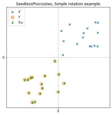
Comparison between SignFlips, OrthogonalProcrustes, SeedlessProcrustes

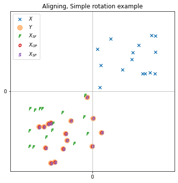
The outcomes of three classes in simple rotation example together are plotted on the same figure in order to allow for a simpler comparison.

fig, ax = plt.subplots(1, 1, figsize=(6, 6))
ax.set_title("Aligning, Simple rotation example")
ax.scatter(X[:,0], X[:,1], label=r"$X$", marker='x')
ax.scatter(Y[:,0], Y[:,1], label=r"$Y$", s=100, alpha=0.5)
ax.scatter(X_prime_SF[:,0],
           X_prime_SF[:,1],
           label=r"$X_{SF}$",
           marker='$F$')
ax.scatter(X_prime_OP[:,0],
           X_prime_OP[:,1],
           label=r"$X_{OP}$", marker='$o$')
ax.scatter(X_prime_SP[:,0],
           X_prime_SP[:,1],
           label=r"$X_{SP}$", marker='$S$')
ax.set(xlim=(-1.20, 1.20), ylim=(-1.20, 1.20))
ax.set_xticks([0])
ax.set_yticks([0])
ax.legend()
ax.grid();

fig, (ax1, ax2, ax3, ax4) = plt.subplots(1, 4, figsize = (16, 4))
heatmap(Q, title=r'$Q$', vmin=-1, vmax=1, ax=ax1)
heatmap(aligner_SF.Q_, title=r'$Q_{SF}$', vmin=-1, vmax=1, ax=ax2)
heatmap(aligner_OP.Q_, title=r'$Q_{OP}$', vmin=-1, vmax=1, ax=ax3)
heatmap(aligner_SP.Q_, title=r'$Q_{SP}$', vmin=-1, vmax=1, ax=ax4);

In this simple example, OrthogonalProcrustes and SeedlessProcrustes align \(X\) to \(Y\) extremply well in terms of the Frobenius norm, whereas SignFlips can only do so well as to bring them to the same quadrant. In fact, when a dataset is a rotated copy of another - OrthogonalProcrustes aligns it up to a numerical epsilon precision.

norm_SignFlips = np.linalg.norm(X_prime_SF - Y)
norm_Orthogonal = np.linalg.norm(X_prime_OP - Y)
norm_Seedless = np.linalg.norm(X_prime_SP - Y)
print('Simple example')
print('Difference in Frobenious norm after Sign Flips ', norm_SignFlips)
print('Difference in Frobenious norm after Orthogonal Procrustes ', norm_Orthogonal)
print('Difference in Frobenious norm after Seedless Procrustes ', norm_Seedless)

Simple example
Difference in Frobenious norm after Sign Flips  1.047909310874878
Difference in Frobenious norm after Orthogonal Procrustes  5.800542824167306e-16
Difference in Frobenious norm after Seedless Procrustes  0.046291889999320164

Shuffled Example

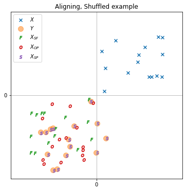
Recall that unlike the other two methods, OrthogonalProcrustes heavily relies on a fact that the vertices of the two datasets are matched. Its performance will deteriorate even on this simple example if the vertices are shuffled, as shown in the following figure.

from sklearn.utils import shuffle

X_shuffled = shuffle(X)

aligner_SF_shuffled = SignFlips()
X_prime_SF_shuffled = aligner_SF_shuffled.fit_transform(X_shuffled, Y)
aligner_OP_shuffled = OrthogonalProcrustes()
X_prime_OP_shuffled = aligner_OP_shuffled.fit_transform(X_shuffled, Y)
aligner_SP_shuffled = SeedlessProcrustes()
X_prime_SP_shuffled = aligner_SP_shuffled.fit_transform(X_shuffled, Y)

fig, ax = plt.subplots(1, 1, figsize=(6, 6))
ax.set_title("Aligning, Shuffled example")
ax.scatter(X_shuffled[:,0], X_shuffled[:,1], label=r"$X$", marker='x')
ax.scatter(Y[:,0], Y[:,1], label=r"$Y$", s=100, alpha=0.5)
ax.scatter(X_prime_SF_shuffled[:,0],
           X_prime_SF_shuffled[:,1],
            label=r"$X_{SF}$", marker='$F$')
ax.scatter(X_prime_OP_shuffled[:,0],
           X_prime_OP_shuffled[:,1],
            label=r"$X_{OP}$", marker='$o$')
ax.scatter(X_prime_SP_shuffled[:,0],
           X_prime_SP_shuffled[:,1],
            label=r"$X_{SP}$", marker='$S$')
ax.set(xlim=(-1.20, 1.20), ylim=(-1.20, 1.20))
ax.set_xticks([0])
ax.set_yticks([0])
ax.legend()
ax.grid();

fig, (ax1, ax2, ax3, ax4) = plt.subplots(1, 4, figsize = (16, 4))
heatmap(Q, title=r'$Q$', vmin=-1, vmax=1, ax=ax1)
heatmap(aligner_SF_shuffled.Q_, title=r'$Q_{SF}$', vmin=-1, vmax=1, ax=ax2)
heatmap(aligner_OP_shuffled.Q_, title=r'$Q_{OP}$', vmin=-1, vmax=1, ax=ax3)
heatmap(aligner_SP_shuffled.Q_, title=r'$Q_{SP}$', vmin=-1, vmax=1, ax=ax4);

In this shuffled example, though the dataset \(X_{shuffled}\) looks the same as dataset \(X\) in the figure, the performance of OthogonalProcrustes is worse than the one in the simple rotation example above. This is because the value of \(i^{th}\) entry in \(X_{shuffled}\) is no longer corresponding with the \(i^{th}\) entry of \(Y\) after being shuffled from \(X\).

Unmatched example

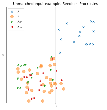
As mentioned above, SeedlessProcrustes can be applied to two datasets with different number of entries. Consider the following example: \(X\) is the same as previous, but the new \(Y\) is a different, larger dataset, generated from the same distribution, and then subsequently rotated.

Y_unmatched = np.random.uniform(0, 1, (30, 2)) @ Q

aligner_SF_unmatched = SignFlips()
X_prime_SF_unmatched = aligner_SF_unmatched.fit_transform(X, Y_unmatched)
aligner_SP_unmatched = SeedlessProcrustes()
X_prime_SP_unmatched = aligner_SP_unmatched.fit_transform(X, Y_unmatched)

fig, ax = plt.subplots(1, 1, figsize=(6, 6))
ax.set_title("Unmatched input example, Seedless Procrustes")
ax.scatter(X[:,0], X[:,1], label=r"$X$", marker='x')
ax.scatter(Y_unmatched[:,0], Y_unmatched[:,1], label=r"$Y$", s=100, alpha=0.5)
ax.scatter(X_prime_SF_unmatched[:,0],
           X_prime_SF_unmatched[:,1],
           label=r"$X_{SF}$",
           marker='$F$')
ax.scatter(X_prime_SP_unmatched[:,0],
           X_prime_SP_unmatched[:,1],
           label=r"$X_{SP}$",
           marker='$S$')
ax.set(xlim=(-1.20, 1.20), ylim=(-1.20, 1.20))
ax.set_xticks([0])
ax.set_yticks([0])
ax.legend()
ax.grid();

fig, (ax1, ax2, ax3) = plt.subplots(1, 3, figsize = (12, 4))
heatmap(Q, title=r'$Q$', vmin=-1, vmax=1, ax=ax1)
heatmap(aligner_SF_unmatched.Q_, title=r'$Q_{SF}$', vmin=-1, vmax=1, ax=ax2)
heatmap(aligner_SP_unmatched.Q_, title=r'$Q_{SP}$', vmin=-1, vmax=1, ax=ax3);

print("Mean of the dataset X:      ", np.mean(X, axis=0))
print("Mean of the dataset Y:      ", np.mean(Y, axis=0))
print("Mean of the dataset X_{SF}: ", np.mean(X_prime_SF_unmatched, axis=0))
print("Mean of the dataset X_{SP}: ", np.mean(X_prime_SP_unmatched, axis=0))

Mean of the dataset X:       [0.58510607 0.48290266]
Mean of the dataset Y:       [-0.4035269 -0.6424252]
Mean of the dataset X_{SF}:  [-0.58510607 -0.48290266]
Mean of the dataset X_{SP}:  [-0.38535747 -0.65348582]

SeedlessProcrustes is still able to align the distributions, while the SignFlips method is only a good heuristic. Note that OthogonalProcrustes is simply inapplicable in this context.