Mixed Membership Stochastic Blockmodel (MMSBM)

import graspologic

import matplotlib.pyplot as plt
import numpy as np
%matplotlib inline

/home/runner/.cache/pypoetry/virtualenvs/graspologic-pkHfzCJ8-py3.10/lib/python3.10/site-packages/tqdm/auto.py:21: TqdmWarning: IProgress not found. Please update jupyter and ipywidgets. See https://ipywidgets.readthedocs.io/en/stable/user_install.html
  from .autonotebook import tqdm as notebook_tqdm

Unlike Stochastic Block Models (SBM), Mixed Membership Stochastic Blockmodels (MMSBM) allow nodes to pertain to multiple communities when interacting with other nodes.

Given a network with \(k\) communities, an MMSBM is parametrized by the number of nodes \(n\) of the graph, a block connectivity matrix \(B \in \mathbb{R}^{k x k}\) where each element specifies the probability of interaction between nodes based upon their community membership, and a vector \(\vec{\alpha}\) which controls the mixed-membership allowed for each node.

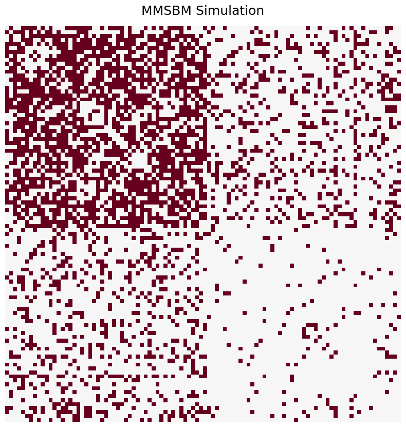
Below, we sample a two-block MMSBM with following parameters:

\begin{align*} n &= 100\\ P &= \begin{bmatrix} 0.7 & 0.2\\ 0.2 & 0.05 \end{bmatrix}\\ \vec{\alpha} &= \begin{bmatrix} 0.1 & 0.1 \end{bmatrix}\\ \end{align*}

from graspologic.simulations import mmsbm

rng = np.random.default_rng(123)

n = 100
p = [[0.7, 0.2],
     [0.2, 0.05]]
alpha = [0.1]*2

G = mmsbm(n, p, alpha, rng = rng)

Visualize the graph using heatmap

from graspologic.plot import heatmap

heatmap(G, cbar= False, title ='MMSBM Simulation');

Generating various types of graphs

Each node \(p\) is assigned a membership vector \(\vec{\pi}_p \in \mathbb{R}^{k}\) sampled from a Dirichlet distribution: \begin{align*} \vec{\pi}_p \sim \mbox{Dir}(\vec{\alpha})\\ \end{align*}

This vector indicates the probability of a node to interact with other nodes as if belonging to a certain community. For example, in a four communities graph, let:

\begin{align*} \vec{\pi}_p &= \begin{bmatrix} 1 & 0 & 0 & 0 \end{bmatrix}\\ \vec{\pi}_q &= \begin{bmatrix} 0.25 & 0.25 & 0.25 & 0.25 \end{bmatrix}\\ \end{align*}

According to \(\vec{\pi}_p\), node \(p\) will always behave as if pertaining to the first community when interacting with other nodes, while node \(q\) will interact 25% of the time as if belonging to community 1, 25% of the time as if belonging to community 2, etc.

Therefore, controlling these membership vectors by varying the parameter \(\vec{\alpha}\) allows generation of various types of graphs.

Generating Erdos-Renyi (ER) graphs

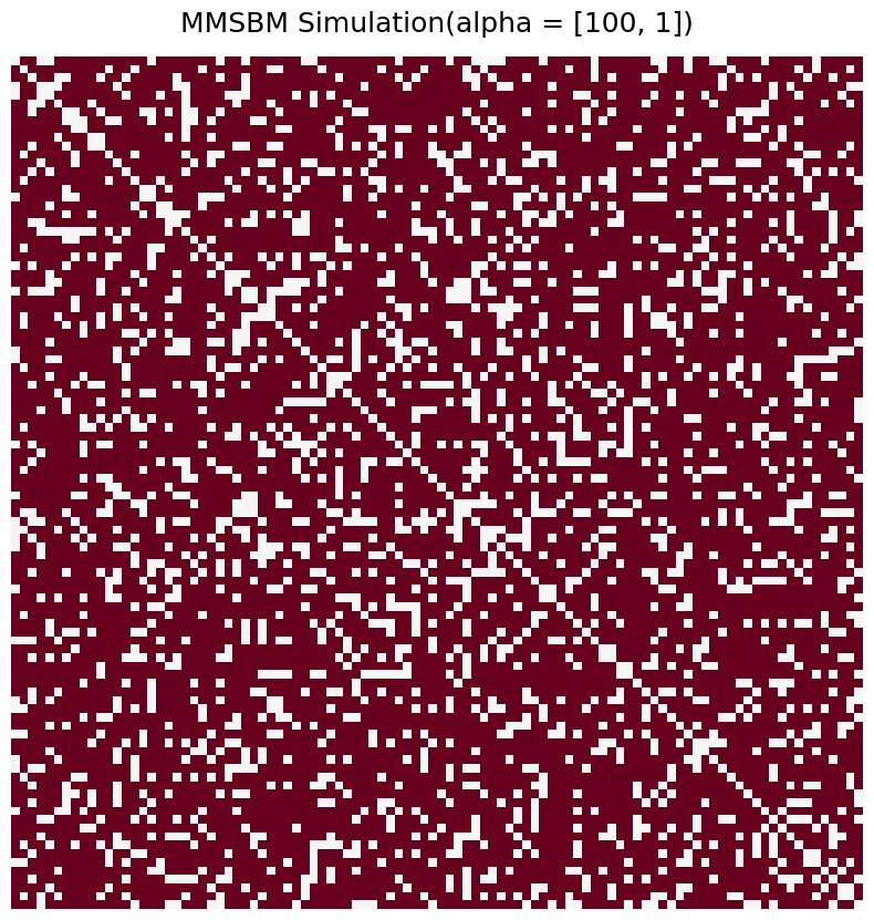
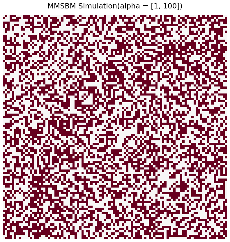
To generate Erdos-Renyi (ER), one of the \(\vec{\alpha}\) entries can be set to be much greater than the others.

For example, consider the two graphs (undirected, no self-loops) parameterized by:

\begin{align*} n &= 100\\ P &= \begin{bmatrix} 0.8 & 0.2\\ 0.2 & 0.5 \end{bmatrix}\\ \end{align*}

With \(\vec{\alpha}\) respectively equal to:

\begin{align*} \vec{\alpha_1} &= \begin{bmatrix} 100 & 1 \end{bmatrix}\\ \vec{\alpha_2} &= \begin{bmatrix} 1 & 100 \end{bmatrix}\\ \end{align*}

from graspologic.simulations import er_np

n = 100
p = [[0.8, 0.2],
     [0.2, 0.5]]

alpha_1 = [100, 1]
G_1 =  mmsbm(n, p, alpha_1, rng = rng)

alpha_2 = [1, 100]
G_2 =  mmsbm(n, p, alpha_2, rng = rng)

Visualize the graphs using heatmap

heatmap(G_1, cbar= False, title ='MMSBM Simulation(alpha = [100, 1])');
heatmap(G_2, cbar= False, title ='MMSBM Simulation(alpha = [1, 100])');

Differences with Stochastic Block Model (SBM) graphs

According to the Stochastic Block Models (SBM), each node in a graph can only pertain to one community. Therefore, one way to recreate such model with an MMSBM is to set all the entries of \(\vec{\alpha}\) equal to the same value. The closer the value is to \(0\) the more the simulated graphs will appear similar to an SBM, the closer the value is to \(1\) the more uniform the graph will look, thus losing the community structure dictated by the SBM.

To show this we sample a four-block SBM (undirected, no self-loops) graph with following parameters: \begin{align*} n &= \begin{bmatrix} 50 & 50 & 50 & 50 \end{bmatrix}\\ B &=\begin{bmatrix} 0.8 & 0.2 & 0.2 & 0.2 \\ 0.2 & 0.8 & 0.2 & 0.2 \\ 0.2 & 0.2 & 0.8 & 0.2 \\ 0.2 & 0.2 & 0.2 & 0.8 \end{bmatrix} \end{align*}

We also sample a four-block MMSBM with parameter \(\vec{\alpha}\) such that: \begin{align*} \vec{\alpha} &= \begin{bmatrix} 0.01 & 0.01 & 0.01 & 0.01 \end{bmatrix}\\ \end{align*}

from graspologic.simulations import sbm

n = [50] * 4
p = [[0.8,0.2,0.2,0.2],
    [ 0.2,0.8,0.2,0.2],
    [ 0.2,0.2,0.8,0.2],
    [ 0.2,0.2,0.2,0.8]]

G_sbm = sbm(n, p, directed=False, loops=False)

n = 200
k = 4
alpha = [0.01]*k

G_mmsbm = mmsbm(n, p, alpha= alpha, rng = rng)

Plot SBM and MMSBM graphs using heatmap

heatmap(G_sbm, cbar= False, title ='SBM Simulation');
heatmap(G_mmsbm, cbar= False, title ='MMSBM Simulation(alpha = 0.01)');

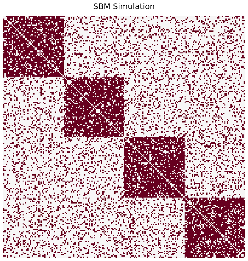
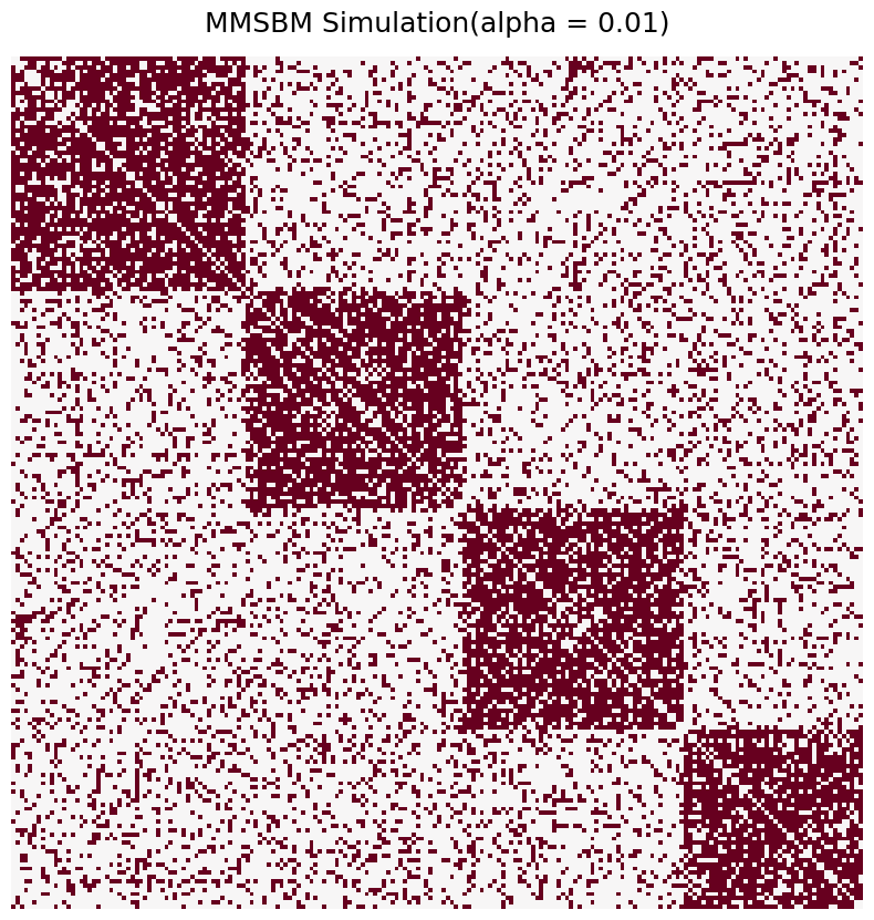
As expected, the two graphs appear to be generated from four-block SBMs with connectivity matrix \(B\). In the MMSBM case, the number of nodes assigned to each block is not specified which is why we can see a different number of nodes per block.

Now let’s try increasing the values of each entry of the concentration parameter \(\vec{\alpha}\) first to \(0.25\), then \(0.5\) and finally to \(1\).

alpha = [0.25]*k
print("First increase alpha to: " + str(alpha))

G_mmsbm_25 = mmsbm(n, p, alpha= alpha, rng = rng)
heatmap(G_mmsbm_25, cbar= False, title ='MMSBM Simulation(alpha = 0.25)');

alpha = [0.5]*k
print("Then increase alpha to: " + str(alpha))

G_mmsbm_50 = mmsbm(n, p, alpha= alpha, rng = rng)
heatmap(G_mmsbm_50, cbar= False, title ='MMSBM Simulation(alpha = 0.5)');

alpha = [1.0]*k
print("Finally increase alpha to: " + str(alpha))

G_mmsbm_100 = mmsbm(n, p, alpha= alpha, rng = rng)
heatmap(G_mmsbm_100, cbar= False, title ='MMSBM Simulation(alpha = 1.0)');

First increase alpha to: [0.25, 0.25, 0.25, 0.25]
Then increase alpha to: [0.5, 0.5, 0.5, 0.5]
Finally increase alpha to: [1.0, 1.0, 1.0, 1.0]

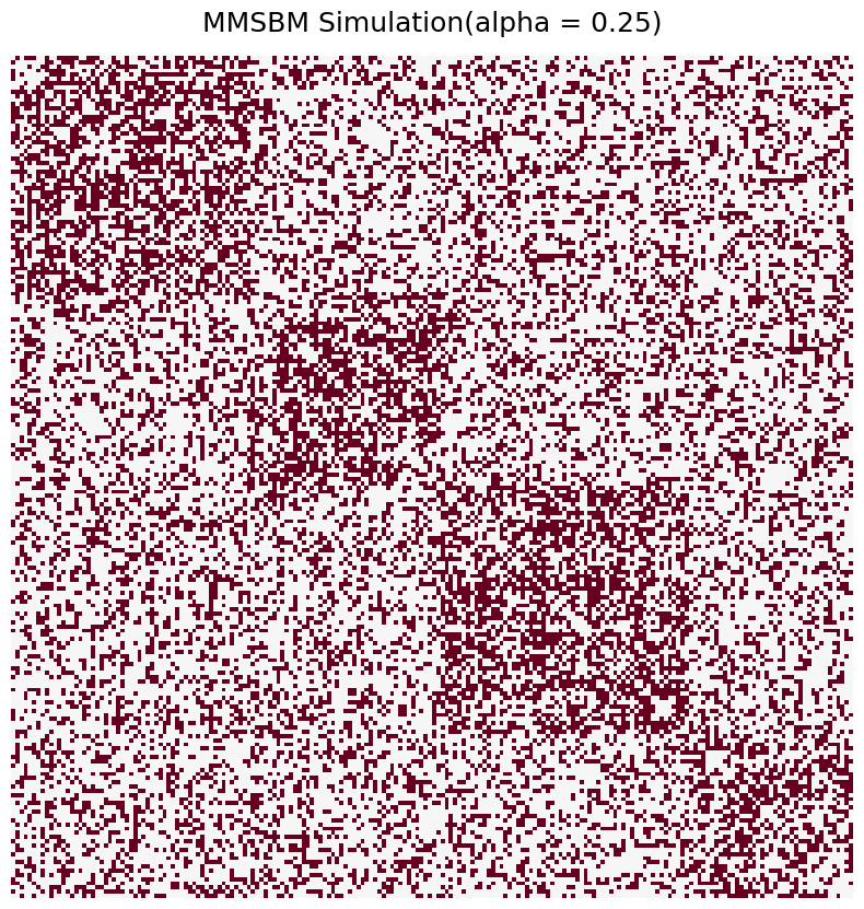
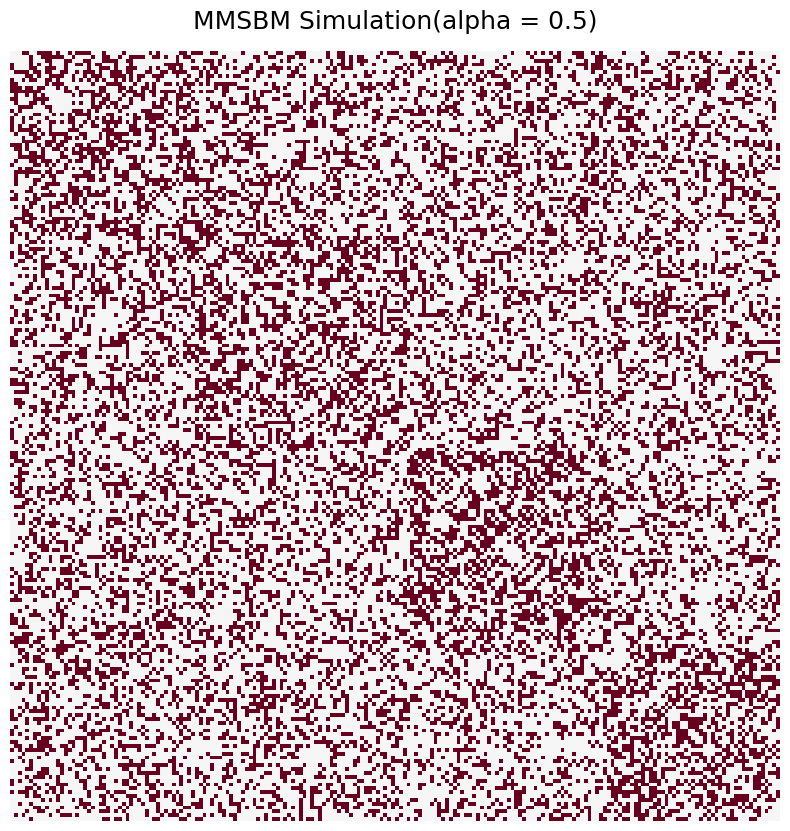
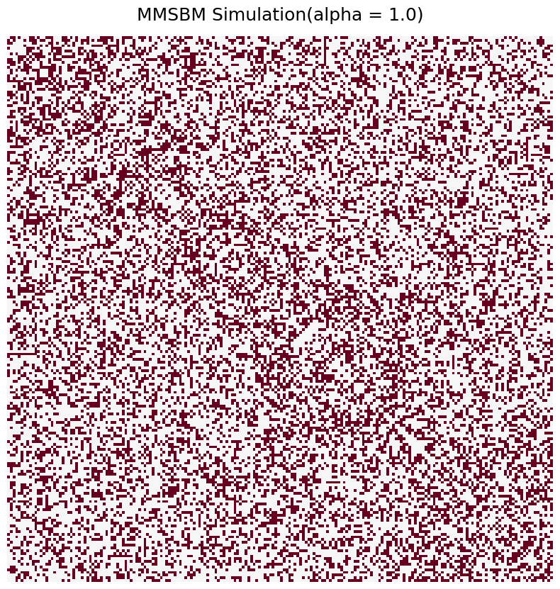
As expected, as we increase the value of \(\vec{\alpha}\) we increase the mixed-membership allowed at each node so that the community structure is progressively lost.