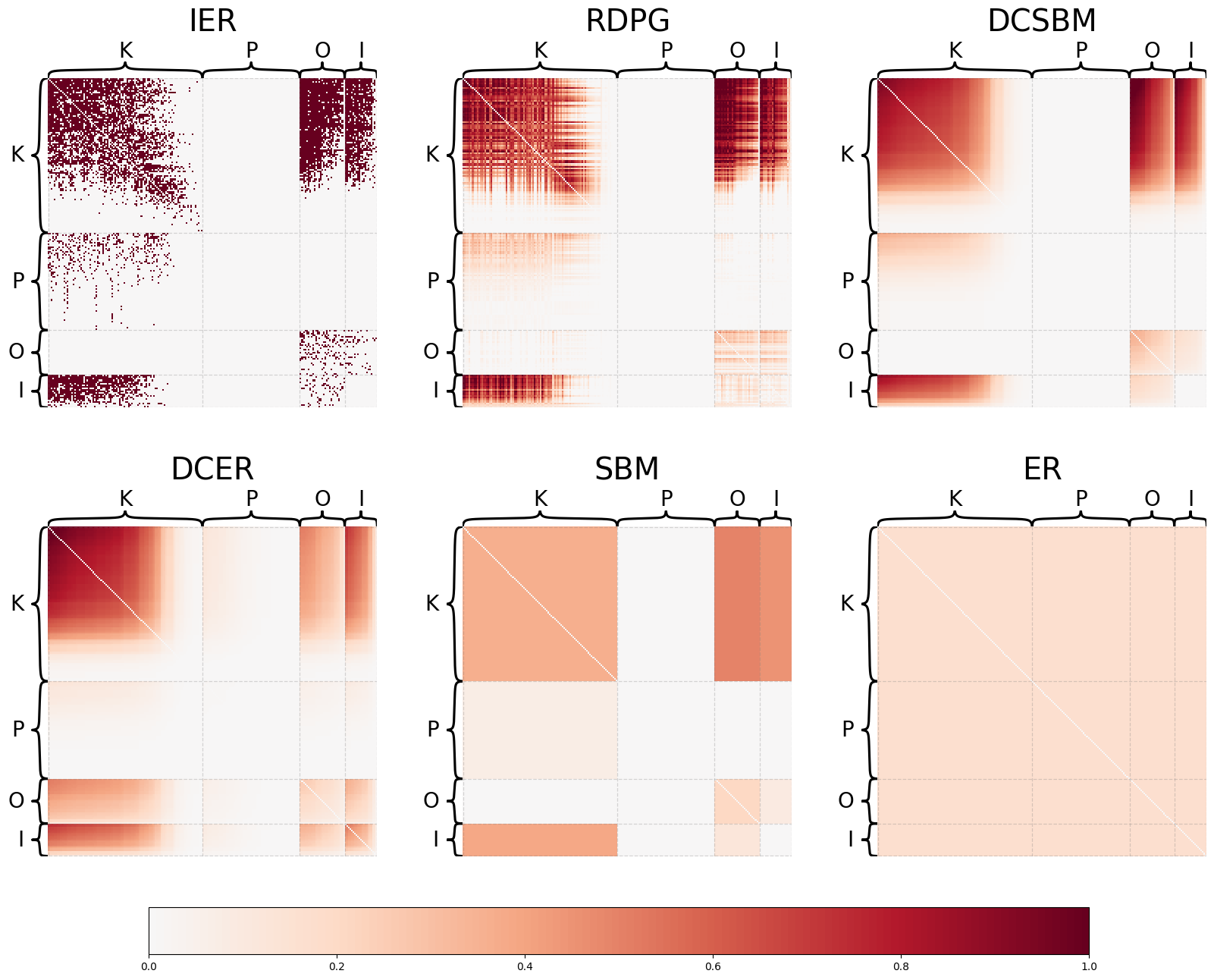
Random Graph Models

This tutorial will introduce the following random graph models:

• Erdos-Reyni (ER)

• Degree-corrected Erdos-Reyni (DCER)

• Stochastic block model (SBM)

• Degree-corrected stochastic block model (DCSBM)

• Random dot product graph (RDPG)

Load some data from graspologic

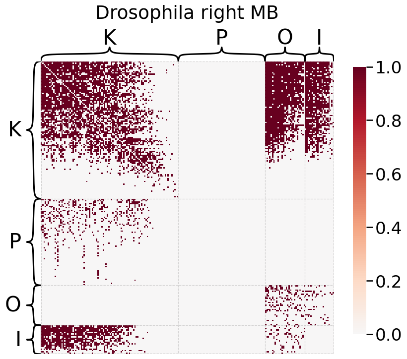
For this example we will use the Drosophila melanogaster larva right mushroom body connectome from Eichler et al. 2017. Here we will consider a binarized and directed version of the graph.

import numpy as np
from graspologic.datasets import load_drosophila_right
from graspologic.plot import heatmap
from graspologic.utils import binarize, symmetrize
%matplotlib inline

adj, labels = load_drosophila_right(return_labels=True)
adj = binarize(adj)
_ = heatmap(adj,
        inner_hier_labels=labels,
        title='Drosophila right MB',
        font_scale=1.5,
        sort_nodes=True)

/home/runner/.cache/pypoetry/virtualenvs/graspologic-pkHfzCJ8-py3.10/lib/python3.10/site-packages/tqdm/auto.py:21: TqdmWarning: IProgress not found. Please update jupyter and ipywidgets. See https://ipywidgets.readthedocs.io/en/stable/user_install.html
  from .autonotebook import tqdm as notebook_tqdm

Preliminaries

\(n\) - the number of nodes in the graph

\(A\) - \(n \times n\) adjacency matrix

\(P\) - \(n \times n\) matrix of probabilities

For the class of models we will consider here, a graph (adjacency matrix) \(A\) is sampled as follows:

\[A \sim Bernoulli(P)\]

While each model we will discuss follows this formulation, they differ in how the matrix \(P\) is constructed. So, for each model, we will consider how to model \(P_{ij}\), or the probability of connection between any node \(i\) and \(j\), with \(i \neq j\) in this case (i.e. no “loops” are allowed for the sake of this tutorial).

---

For each graph model we will show:

• how the model is formulated

• how to fit the model using graspologic

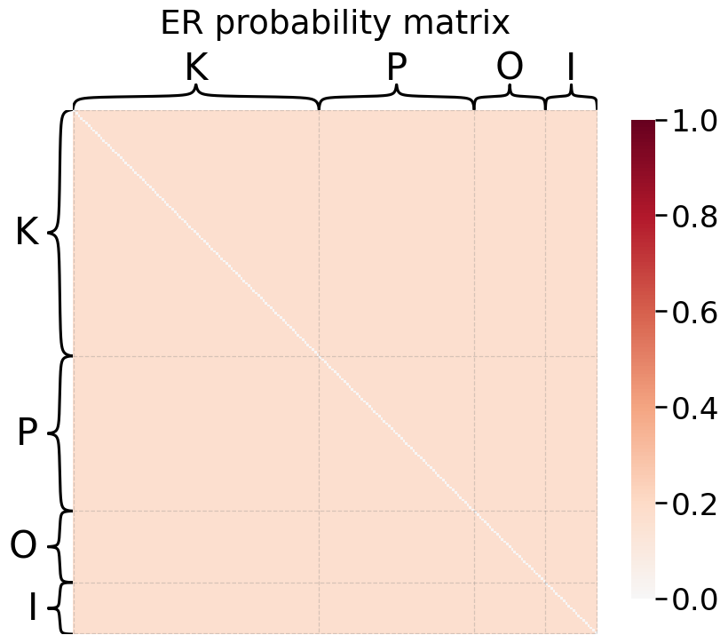
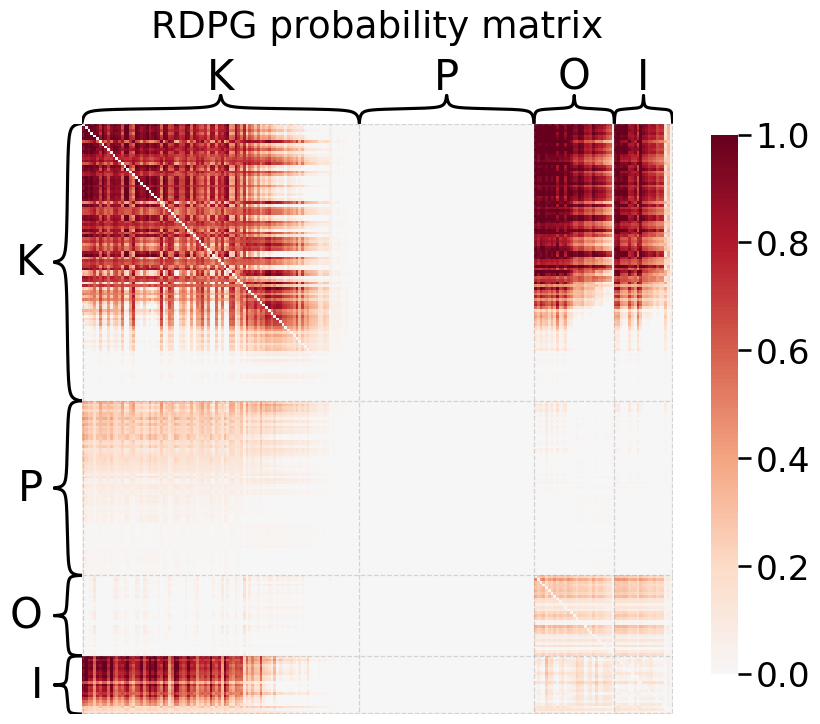
• the P matrix that was fit by the model

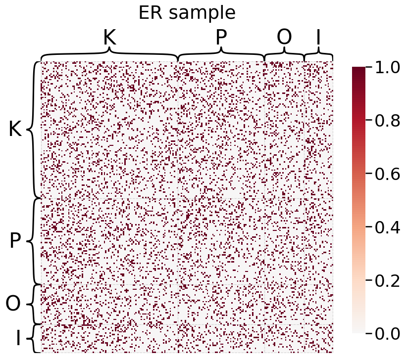
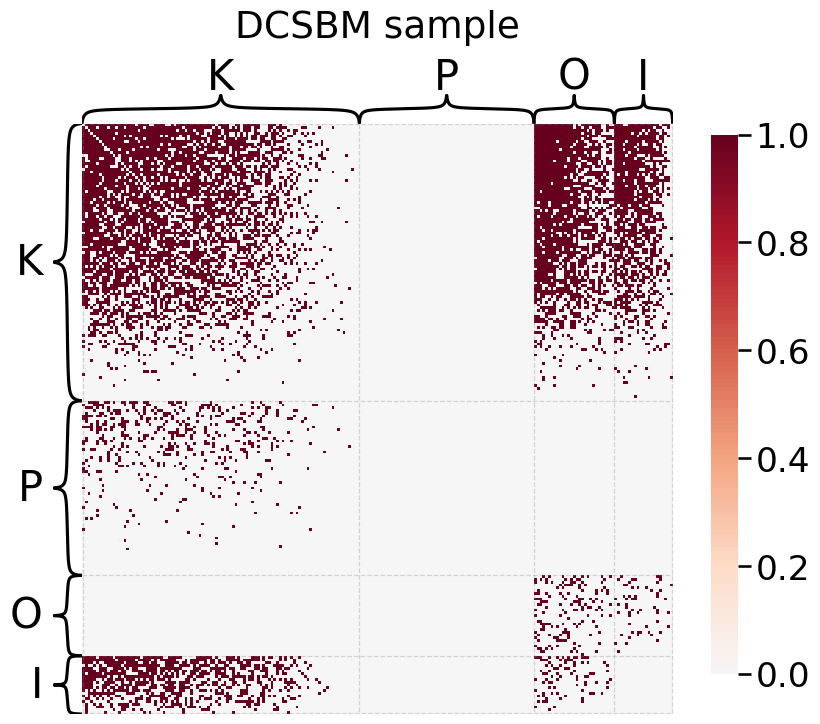
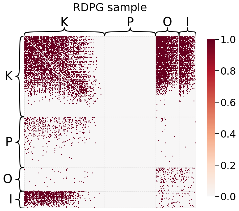
• a single sample from the fit model

Erdos-Reyni (ER)

The Erdos-Reyni (ER) model is the simplest random graph model. We are interested in modeling the probability of an edge existing between any two nodes, \(i\) and \(j\). We denote this probability \(P_{ij}\). For the ER model:

\[P_{ij} = p\]

for any combination of \(i\) and \(j\).

This means that the one parameter \(p\) is the overall probability of connection for any two nodes.

from graspologic.models import EREstimator
er = EREstimator(directed=True,loops=False)
er.fit(adj)
print(f"ER \"p\" parameter: {er.p_}")
heatmap(er.p_mat_,
        inner_hier_labels=labels,
        font_scale=1.5,
        title="ER probability matrix",
        vmin=0, vmax=1,
        sort_nodes=True)
_ = heatmap(er.sample()[0],
        inner_hier_labels=labels,
        font_scale=1.5,
        title="ER sample",
        sort_nodes=True)

ER "p" parameter: 0.16688812117990964

Degree-corrected Erdos-Reyni (DCER)

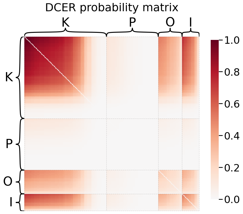
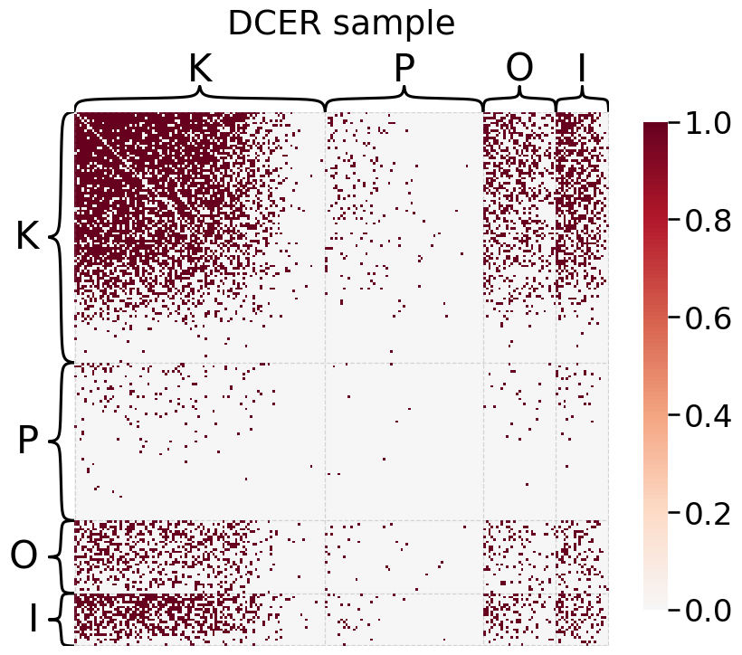
A slightly more complicated variant of the ER model is the degree-corrected Erdos-Reyni model (DCER). Here, there is still a global parameter \(p\) to specify relative connection probability between all edges. However, we add a promiscuity parameter \(\theta_i\) for each node \(i\) which specifies its expected degree relative to other nodes:

\[P_{ij} = \theta_i \theta_j p\]

so the probability of an edge from \(i\) to \(j\) is a function of the two nodes’ degree-correction parameters, and the overall probability of an edge in the graph.

from graspologic.models import DCEREstimator
dcer = DCEREstimator(directed=True,loops=False)
dcer.fit(adj)
print(f"DCER \"p\" parameter: {dcer.p_}")
heatmap(dcer.p_mat_,
        inner_hier_labels=labels,
        vmin=0,
        vmax=1,
        font_scale=1.5,
        title="DCER probability matrix",
        sort_nodes=True);
_ = heatmap(dcer.sample()[0],
        inner_hier_labels=labels,
        font_scale=1.5,
        title="DCER sample",
        sort_nodes=True)

DCER "p" parameter: 7536.0

Stochastic block model (SBM)

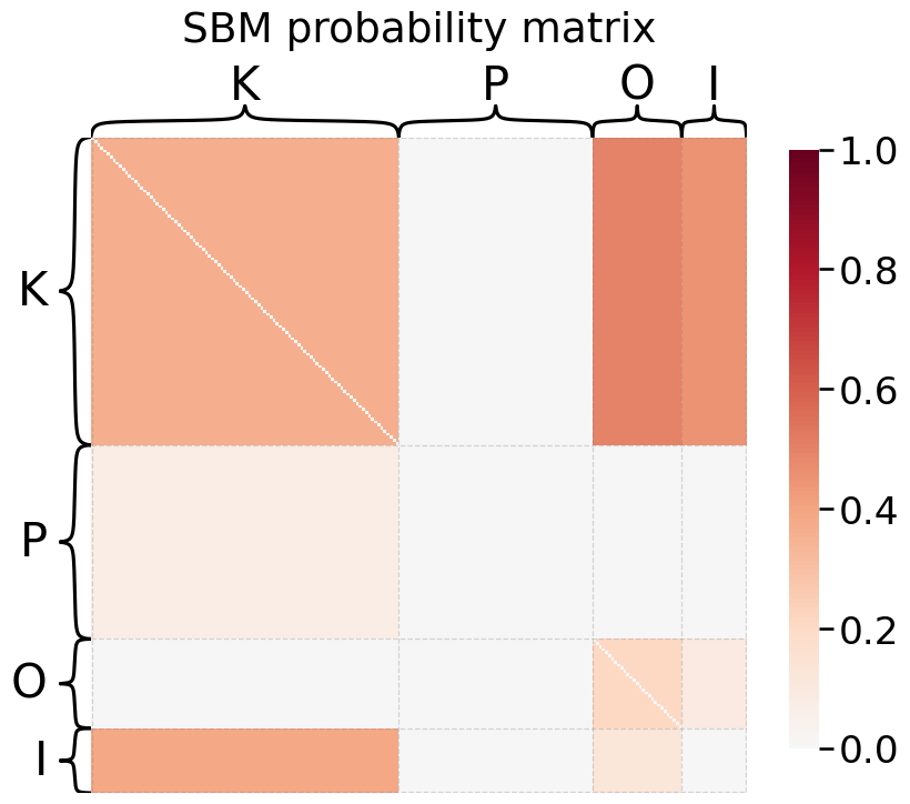
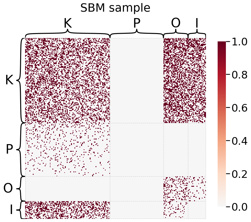
Under the stochastic block model (SBM), each node is modeled as belonging to a block (sometimes called a community or group). The probability of node \(i\) connecting to node \(j\) is simply a function of the block membership of the two nodes. Let \(n\) be the number of nodes in the graph, then \(\tau\) is a length \(n\) vector which indicates the block membership of each node in the graph. Let \(K\) be the number of blocks, then \(B\) is a \(K \times K\) matrix of block-block connection probabilities.

\[P_{ij} = B_{\tau_i \tau_j}\]

from graspologic.models import SBMEstimator
sbme = SBMEstimator(directed=True,loops=False)
sbme.fit(adj, y=labels)
print("SBM \"B\" matrix:")
print(sbme.block_p_)
heatmap(sbme.p_mat_,
        inner_hier_labels=labels,
        vmin=0,
        vmax=1,
        font_scale=1.5,
        title="SBM probability matrix",
        sort_nodes=True)
_ = heatmap(sbme.sample()[0],
        inner_hier_labels=labels,
        font_scale=1.5,
        title="SBM sample",
        sort_nodes=True)

SBM "B" matrix:
[[0.         0.38333333 0.11986864 0.        ]
 [0.44571429 0.3620202  0.49448276 0.        ]
 [0.09359606 0.         0.20812808 0.        ]
 [0.         0.07587302 0.         0.        ]]

Degree-corrected stochastic block model (DCSBM)

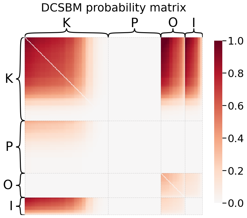
Just as we could add a degree-correction term to the ER model, so too can we modify the stochastic block model to allow for heterogeneous expected degrees. Again, we let \(\theta\) be a length \(n\) vector of degree correction parameters, and all other parameters remain as they were defined above for the SBM:

\[P_{ij} = \theta_i \theta_j B_{\tau_i, \tau_j}\]

Note that the matrix \(B\) may no longer represent true probabilities, because the addition of the \(\theta\) vectors introduces a multiplicative constant that can be absorbed into the elements of \(\theta\).

from graspologic.models import DCSBMEstimator
dcsbme = DCSBMEstimator(directed=True,loops=False)
dcsbme.fit(adj, y=labels)
print("DCSBM \"B\" matrix:")
print(dcsbme.block_p_)
heatmap(dcsbme.p_mat_,
        inner_hier_labels=labels,
        font_scale=1.5,
        title="DCSBM probability matrix",
        vmin=0,
        vmax=1,
        sort_nodes=True)
_ = heatmap(dcsbme.sample()[0],
        inner_hier_labels=labels,
        title="DCSBM sample",
        font_scale=1.5,
        sort_nodes=True)

DCSBM "B" matrix:
[[   0.  805.   73.    0.]
 [ 936. 3584. 1434.    0.]
 [  57.    0.  169.    0.]
 [   0.  478.    0.    0.]]

Random dot product graph (RDPG)

Under the random dot product graph model, each node is assumed to have a “latent position” in some \(d\)-dimensional Euclidian space. This vector dictates that node’s probability of connection to other nodes. For a given pair of nodes \(i\) and \(j\), the probability of connection is the dot product between their latent positions. If \(x_i\) and \(x_j\) are the latent positions of nodes \(i\) and \(j\), respectively:

\[P_{ij} = \langle x_i, x_j \rangle\]

from graspologic.models import RDPGEstimator
rdpge = RDPGEstimator(loops=False)
rdpge.fit(adj, y=labels)
heatmap(rdpge.p_mat_,
        inner_hier_labels=labels,
        vmin=0,
        vmax=1,
        font_scale=1.5,
        title="RDPG probability matrix",
        sort_nodes=True
       )
_ = heatmap(rdpge.sample()[0],
        inner_hier_labels=labels,
        font_scale=1.5,
        title="RDPG sample",
        sort_nodes=True)

Create a figure combining all of the models

import matplotlib as mpl
import matplotlib.pyplot as plt
import seaborn as sns
from matplotlib import cm
from matplotlib.pyplot import get_cmap

fig, axs = plt.subplots(2, 3, figsize=(20, 16))

# colormapping
cmap = get_cmap("RdBu_r")

center = 0
vmin = 0
vmax = 1
norm = mpl.colors.Normalize(0, 1)
cc = np.linspace(0.5, 1, 256)
cmap = mpl.colors.ListedColormap(cmap(cc))

# heatmapping
heatmap_kws = dict(
    inner_hier_labels=labels,
    vmin=0,
    vmax=1,
    cbar=False,
    cmap=cmap,
    center=None,
    hier_label_fontsize=20,
    title_pad=45,
    font_scale=1.6,
    sort_nodes=True
)

models = [rdpge, dcsbme, dcer, sbme, er]
model_names = ["RDPG", "DCSBM","DCER", "SBM", "ER"]

heatmap(adj, ax=axs[0][0], title="IER", **heatmap_kws)
heatmap(models[0].p_mat_, ax=axs[0][1], title=model_names[0], **heatmap_kws)
heatmap(models[1].p_mat_, ax=axs[0][2], title=model_names[1], **heatmap_kws)
heatmap(models[2].p_mat_, ax=axs[1][0], title=model_names[2], **heatmap_kws)
heatmap(models[3].p_mat_, ax=axs[1][1], title=model_names[3], **heatmap_kws)
heatmap(models[4].p_mat_, ax=axs[1][2], title=model_names[4], **heatmap_kws)


# add colorbar
sm = plt.cm.ScalarMappable(cmap=cmap, norm=norm)
sm.set_array(dcsbme.p_mat_)
_ = fig.colorbar(sm,
             ax=axs,
             orientation="horizontal",
             pad=0.04,
             shrink=0.8,
             fraction=0.08,
             drawedges=False)